The ssWavelets Package: Wavelet Functionality for Package sampSurf

Overview of the ssWavelets package

The ssWavelets package is meant to be used in conjunction with the sampSurf package to perform wavelet decomposition on the results of a sampling surface simulation. It provides an S4 class structure with constuctor or generator functions that are tailored to work specifically on objects of class sampSurf. Currently, the only supported decomposition is the maximal overlap discrete wavelet transform (MODWT), although the class structure established will allow for extensions if other decompositions are desired in the future. In addition, only the Haar wavelet filter is supported currently, although, since the underlying wavelet code used in the package (waveslim) supports other filters, support for these could also be added in the future.

In general, the wavelet filter decomposes the sampSurf simulation results by scale (distance), with each scale corresponding to a different level of the decomposition. This results in a set of anisotropic wavelet coefficients for each scale or level, one each for horizontal, vertical and diagonal components; the sum of these yields an isotropic decomposition for that scale. Residual smooth coefficients for the coarsest level are also available from applying the scaling filter, and its mean corresponds to the sample mean of the sampling surface from sampSurf. Interesting as these raw wavelet decompositions may be, the main interest of the wavelet analysis from a sampling perspective has to do with the sample variance, which is the sampling surface variance from a simulation run of sampSurf. The different wavelet decomposition variances corresponding to the raw wavelet coefficients can be easily constructed at each level from the coefficients and are included as part of object creation. These wavelet variances also correspond to a decomposition of the sample variance, or, its total or average energy, depending upon the particular level, filter, and use. Covariance analysis, which may prove useful in the comparison of sampling methods at different scales, is also available in the package.

Details of package use are found in the package vignette: A User's Guide to the ssWavelets Package, while the help system is detailed in the normal package vignette. Information on installation and a simple example are found in the following sections. Please refer to the vignettes for more details.

ssWavelets installation

Before installing ssWavelets it is recommended that you first install sampSurf and its dependancies. Please refer to the sampSurf Installation section of its webpage for installation instructions pertaining to that package.

ssWavelets is available only on R-Forge. On the project pages, you will note that you can install the package directly from R-Forge using…

install.packages("ssWavelets", repos="http://R-Forge.R-project.org")

and can include the dep=TRUE argument if you want the packages that ssWavelets is dependent upon to also be installed. However, this is not recommended, please see the reasons in the above link (sampSurf installation) for more details.

In addition, the ssWavelets package requires that the following package be installed prior to use. It is best to install the most recent version from CRAN as…

install.packages("waveslim")

ssWavelets package vignette

As noted above, there is one extra package vignette (aside from the default help vignette) distributed with the package itself. Both can also be downloaded here from the R-Forge versions if desired…

The following gives another simple application of wavelets to sampling surfaces…

Gove, J. H., 2017. Some Refinements on the Comparison of Areal Sampling Methods via Simulation. Forests 8, 393:1-24; doi:10.3390/f8100393.

ssWavelet examples

Here we present one very simple example illustrating how to use a few of the main functions in the ssWavelets package. The User's Guide vignette goes into extensive detail concerning the use of the methods shown below as well as many others. In addition, the online help system is quite thorough in documenting class structures, generic functions, and their methods. Therefore, what is provided is a very terse example to show a little of the functionality of the package here. Please refer to the sampSurf Examples and associated vignettes for more information on constructing sampling surfaces.

Critical Height Sampling

The following code will generate a volume sampling surface using critical height sampling (CHS) in the form of a sampSurf object that will be the subject of the subsequent wavelet variance decomposition. A similar example, but with a different tree population and more details is found in the User's Guide. The metric system is used by default.

R> require(sampSurf)
R> tract.m = Tract(c(x = 64, y = 64), cellSize=1) #square tract, dyadic grid ~0.5ha
R> buffTr.m = bufferedTract(bufferWidth = 10, tract.m)
R> ag3m = angleGauge(3) #metric
R> sschs = sampSurf(25, buffTr.m, iZone = 'criticalHeightIZ', angleGauge = ag3m, dbhs = c(12,30),
+                  topDiam = c(0,0), startSeed = 304, referenceHeight = 'dbh')

Number of trees in collection = 25
Heaping tree: 1,2,3,4,5,6,7,8,9,10,11,12,13,14,15,16,17,18,19,20,21,22,23,24,25,

R> plot(sschs, useImage = FALSE)

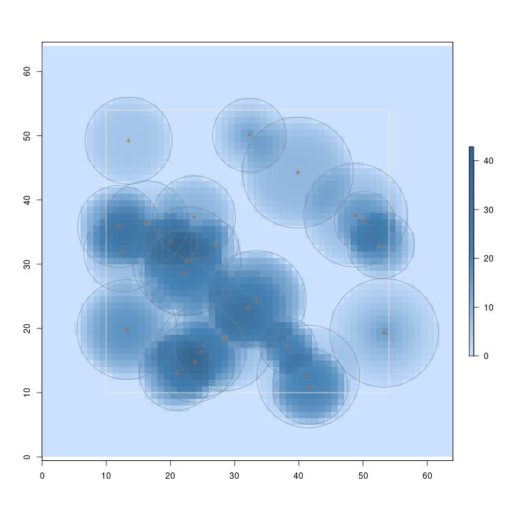
The above figure presents the volume sampling surface for CHS. Note how the surface (volume estimate) varies within each tree's inclusion zone, depending on its dimensions.

Now we can do a MODWT analysis on this surface…

R> J.chs = 5                             #highest decomposition level: J_0
R> chs.modwt = ssMODWT(sschs, J = J.chs)

Inclusion zone class: criticalHeightIZ
Surface variance = 75.792717
Wavelet variance = 75.774213 (MODWT)
Surf/Wave var ratio = 1.0002442
Check: surface var matrix = 75.774213 = E[X^2] - E[X]^2
Surface mean = 6.0179401
Wavelet mean = 6.0179401 (MODWT)
Wavelet mean = 6.01794 (MRA)

R> plotLevel2D(chs.modwt, type = 'var', level = 1, decompType = 'modwt')

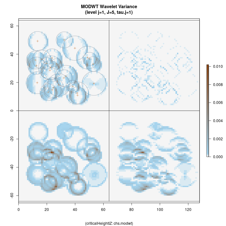
Top left: horizontal
Top right: diagonal
Bottom right: vertical
Botton left: isotropic

The figure above shows the four anisotropic variance decompositions at level j=1, corresponding to the legend printed below the figure. This first-level decomposition is good for edge detection and essentially picks out the edges of the inclusion zone as the wavelet traverses the surface in the desired orientation. But as can be seen, it also picks out areas within individual or overlapping inclusion zones where the surface values change more than others. If this were compared against a surface using horizontal point sampling, each tree's surface would be a cylinder, and the edges would be the main feature at this scale. The isotropic image (bottom left) combines the tree anisotropic views.

The raw wavelet coefficients are shown in the following figure for comparison. Here we can see how positive coefficients are generated as the wavelet encounters the boundary of an inclusion zone coming from a background value (of zero), or more generally as the surface increases in the direction of the wavelet filter. Conversely, negative values are generated as the surface decreases in the same direction as the filter.

R> plotLevel2D(chs.modwt, type = 'raw', level = 1, decompType = 'modwt')

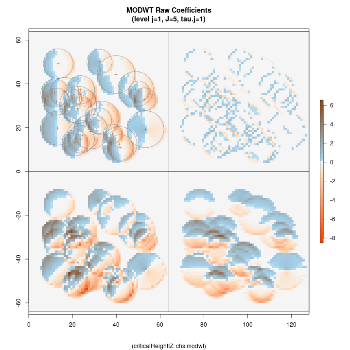
Top left: horizontal
Top right: diagonal
Bottom right: vertical
Botton left: isotropic

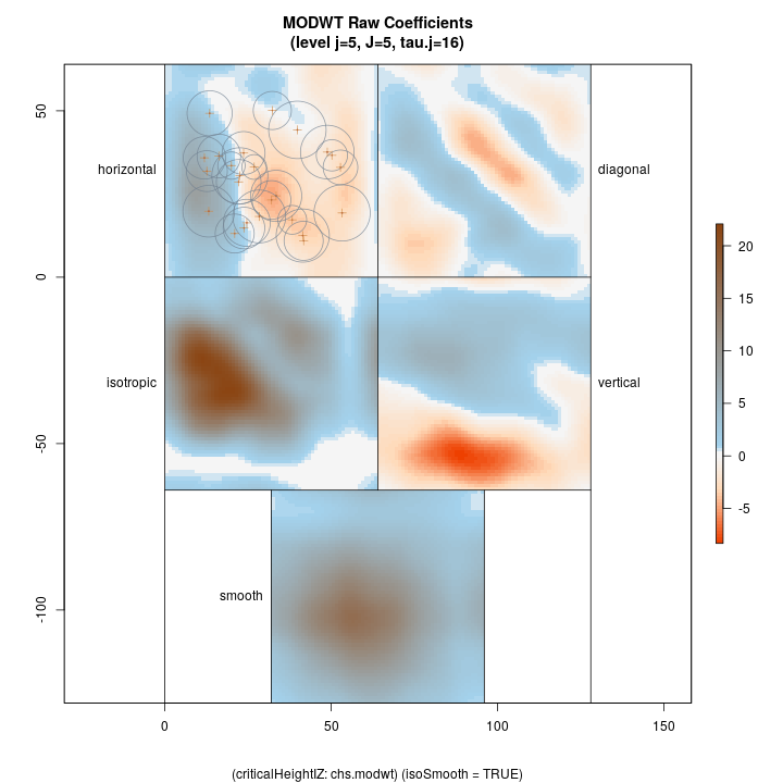
Lastly, we show the coarsest level decomposition for both the variance and raw coefficients, respectively. Note that the final image is of the smooth; these images show larger scale relations…

R> plotLevel2D(chs.modwt, type = 'var', level = J.chs, decompType = 'modwt')

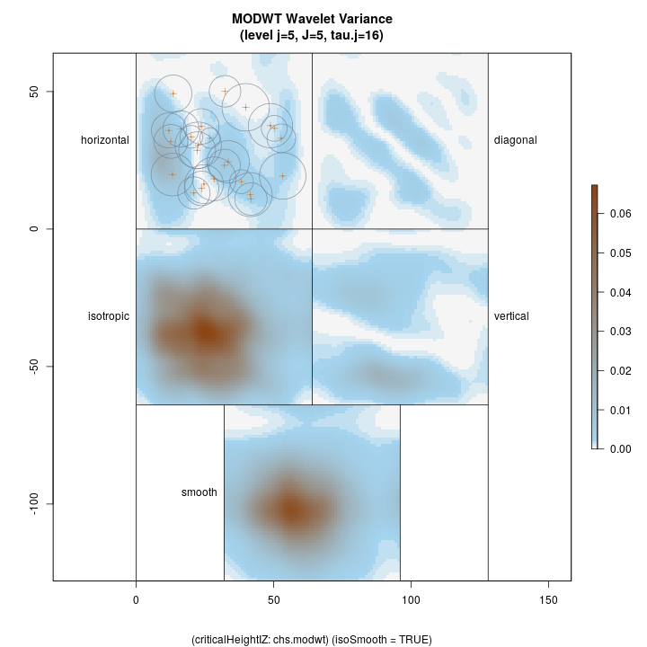
Top left: horizontal
Top right: diagonal
Bottom right: vertical
Botton left: isotropic
Bottom middle: final smooth

R> plotLevel2D(chs.modwt, type = 'raw', level = J.chs, decompType = 'modwt', runQuiet = TRUE)

Summary

There are many more aspects to this package as outlined in the User's Guide. These include plotting functions that allow the comparision of different sampling methods by scale and covariance analysis. It also describes the edge or boundary correction methods available in the wavelet analyis phase.